Neural Contextual Bandits with TensorFlow: A Deep Learning Approach to In-App Purchase Recommendations

Abstract: This article details the implementation of a Neural Contextual Bandit system for optimizing In-App Purchases in mobile games. By transitioning from traditional linear models to a Deep Q-Network architecture, we address the challenge of sparse reward signals in Free-to-Play economies. Technical contributions include a GPU-accelerated preprocessing graph to eliminate CPU-GPU bottlenecks, the adoption of Binary Focal Loss to handle reward-class imbalance (>95% negatives), and an off-policy learning pipeline for production logs. These architectural improvements yielded a 109% increase in ranking quality (AUC-ROC rising from 0.35 to 0.7311) compared to the baseline model made by Google Firebase.

---

⚠️ Important: Any views, material or statements expressed are mines and not those of my employer, read the disclaimer to learn more.¹

🚀 Access the source code from Github, available here.

---

1. Introduction: The Business Case for Personalized IAP

1.1 The “Free-to-Play” Monetization Paradox

In the $103B+ mobile gaming industry (Newzoo, 2025), the “Free-to-Play” (F2P) model over other markets, yet it presents a paradox: while millions play, only a fraction pay. Industry benchmarks consistently show that In-App Purchase (IAP) conversion rates typically hover between 2% and 5%. This means that for every 100 users acquired, often at a cost (CPI) ranging from $1 to $5+ per user, 95 to 98 of them will never generate direct revenue.

Historically, developers relied on “Whales” (the top 1-2% of spenders) to drive monetization (Sifa et al., 2018, p. 3). However, this strategy is becoming increasingly obsolete, as user acquisition costs rise and privacy regulations like IDFA depreciation limit targeting, so firms must adopt a “customer-centric approach” to survive in a privacy-first world (McKinsey & Company, 2021). The “missed opportunity” of the remaining ~97% becomes the central problem to solve, since they still represent ~50% of the total revenue (Sifa et al., 2018, p. 4).

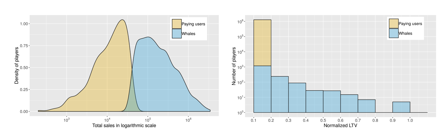
Density function from the kernel density and normalized distribution of total in-app revenue (Sifa et al., 2018, p. 4)

1.2 The Missed Opportunity: Relevance vs. Churn

The primary lever to unlock revenue from the non-paying majority is contextual relevance. A “Coin Multiplier” might be tempting to a competitive player on a losing streak, while an “Extra Life” appeals to a casual player stuck on a hard level.

However, getting this wrong carries significant risk. Static, rule-based systems often fail by showing irrelevant or overpriced offers, which can actively drive players away. A study published by Harvard Business School on Game Design highlights this issue, revealing a 0.880 correlation between level difficulty and user churn. So, there is a positive correlation of 0.394 between level difficulty and the likelihood of a player churning within the first 30 days (Ascarza, Netzer, & Runge, 2024, p. 19).

This also can conclude that an irrelevant offer (e.g., a cosmetic item) shown during a moment of high frustration is not just a missed sale, it’s a retention risk. Then the challenge, is to dynamically match the right offer to the right user at the right price point in real-time. So, solving this requires moving beyond simple A/B testing or linear segmentation; it demands a system that can learn complex patterns, non-linear relationships between user behavior (session length, difficulty, device type) and purchase intent; a perfect use-case for Neural Contextual Bandits (RecSys).

1.3 Contextual Bandits in Recommendation Systems

As highlighted by a Columbia reaserch on RL (Wang et al., 2019), this kind of algorithms represent a fundamental framework for balancing exploration and exploitation in recommendation systems. Unlike traditional multi-armed bandits, contextual bandits leverage user context (demographics, behavior, device characteristics) to make personalized action selections. The core challenge lies in learning a policy $\pi: \mathcal{X} \rightarrow \mathcal{A}$ that maps contexts $x \in \mathcal{X}$ to actions $a \in \mathcal{A}$ to maximize cumulative reward (expected $\mathbb{E}$):

$\max_{\pi} \mathbb{E}\left[\sum_{t=1}^{T} r_t(a_t, x_t)\right]$

where $r_t$ denotes the reward at time step $t$, and $a_t = \pi(x_t)$ is the action selected based on context $x_t$.

1.4 Limitations of Traditional Approaches

Traditional contextual bandit algorithms, such as LinUCB (Li et al., 2012) and Thompson Sampling with linear models, face significant limitations in modern recommendation systems:

1. Linear Model Assumptions: LinUCB uses ridge regression, which assumes linear relationships between features and rewards, a critical limitation that prevents capturing complex non-linear interactions. E.g., price elasticity the relationship between action (power-up) price and purchase probability have non-linear behavior. In real-world scenarios, price sensitivity follows a logarithmic inverse relationship (e.g., $\text{sensitivity} = 1 / \log(1 + \text{price})$), where small price changes at low price points have disproportionately larger effects than equivalent changes at high price points, factor simulated here.

2. Scalability Constraints: As the action space grows (e.g., 8+ distinct powerups) and feature dimensionality increases, linear models require explicit feature engineering to maintain performance, increasing development and maintenance costs.

3. Cold Start Problem: Linear models struggle with sparse data scenarios common in gaming applications, where new users or rare action combinations provide insufficient signal for reliable parameter estimation.

4. Off-Policy Learning Challenges: Real-world recommendation systems must learn from historical logs generated by previous policies (off-policy learning). Linear models often fail to generalize beyond the logging policy’s current action distribution, and will be blinded if a new action is inserted. On the opposite side neural networks are flexible and suitable for contextual bandit problems with high dimensional feature mappings (Zhou et al. 2020, p. 1).

1.6 Solution Proposed

To address the limitations of traditional linear models and allow for scalable production deployment, this implementation is guided by 3 primary hypotheses regarding theoretical grounding, system architecture, and optimization objectives.

1.6.1 Theoretical Foundation

This approach derives its framework from the “Part II - Neural Contextual Bandits” lectures outlined by Ban, Qi, & He in their work on personalized recommendation (Ban et al., 2023). We will work under the hypothesis that deep neural networks can serve as effective function approximators for the policy $\pi^*$ in contextual bandit settings, capturing the non-linear dynamics that LinUCB misses.

1.6.2 Engineering Foundation

From an implementation perspective, we hypothesize that the primary bottleneck in modern production recommender systems is not model inference time, but the CPU-to-GPU data transfer overhead caused by external preprocessing.

Therefore, the goal is to construct a Deep Neural Network where feature engineering is not a separate step, but a Graph of Preprocessing Layers within the TensorFlow graph. By calculating and persisting static components (like Vocabulary and Weights) before computation, we eliminate runtime bottlenecks and training-serving skew.

1.6.3 Optimization Foundation

Finally, we change the standard use of MSE and Accuracy for IAP optimization, proposing that Binary Focal Loss and AUC are better for this specific domain:

Binary Focal Loss vs. MSE:

• Optimizer Perspective: In a dataset where 95%+ of samples are negatives (no purchase), MSE is easily minimized by predicting “zero” for everything, leading to vanishing gradients for the rare positive signals. Focal Loss dynamically scales the loss based on prediction confidence, effectively “down-weighting” the easy negatives and keeping the optimizer focused on the hard, sparse positive examples.
• Business Perspective: Minimizing average error is irrelevant if the model misses the “Whales” (discussed in 1.1). We need a loss function that prioritizes finding the “needle in the haystack” (the purchaser) rather than correctly predicting that a non-payer won’t pay.

AUC vs. Accuracy:

• Math Perspective: In an imbalanced dataset (e.g., 5% conversion), a “simpler” model that predicts “no purchase” for everyone achieves 95% accuracy but learns nothing.
• Business Perspective: The goal of an IAP system is rarely binary classification; it is Ranking. We have limited screen real estate (often just one pop-up slot). AUC measures the probability that the model ranks a randomly chosen positive instance higher than a randomly chosen negative one, where a high value guarantees that when the system decides to intervene, it is presenting the offer with the highest relative probability of conversion, which is the direct driver of revenue.

2. System Architecture

2.1 Overview

This implementation follows a modular architecture that separates preprocessing, model training, and inference into distinct, reusable components. The system is built entirely on TensorFlow 2.17.1 and Keras 3.0.

The architecture consists of 2 primary submodels:

• Preprocessing Submodel: A functional Keras model made of graph of layers, that handles feature encoding, normalization, and action mapping. This submodel is adapted to the dataset during initialization and persists vocabulary mappings for consistent inference.

• Q-Network (MLP): A deep multi-layer perceptron that estimates Q-values for each action given the preprocessed context features.

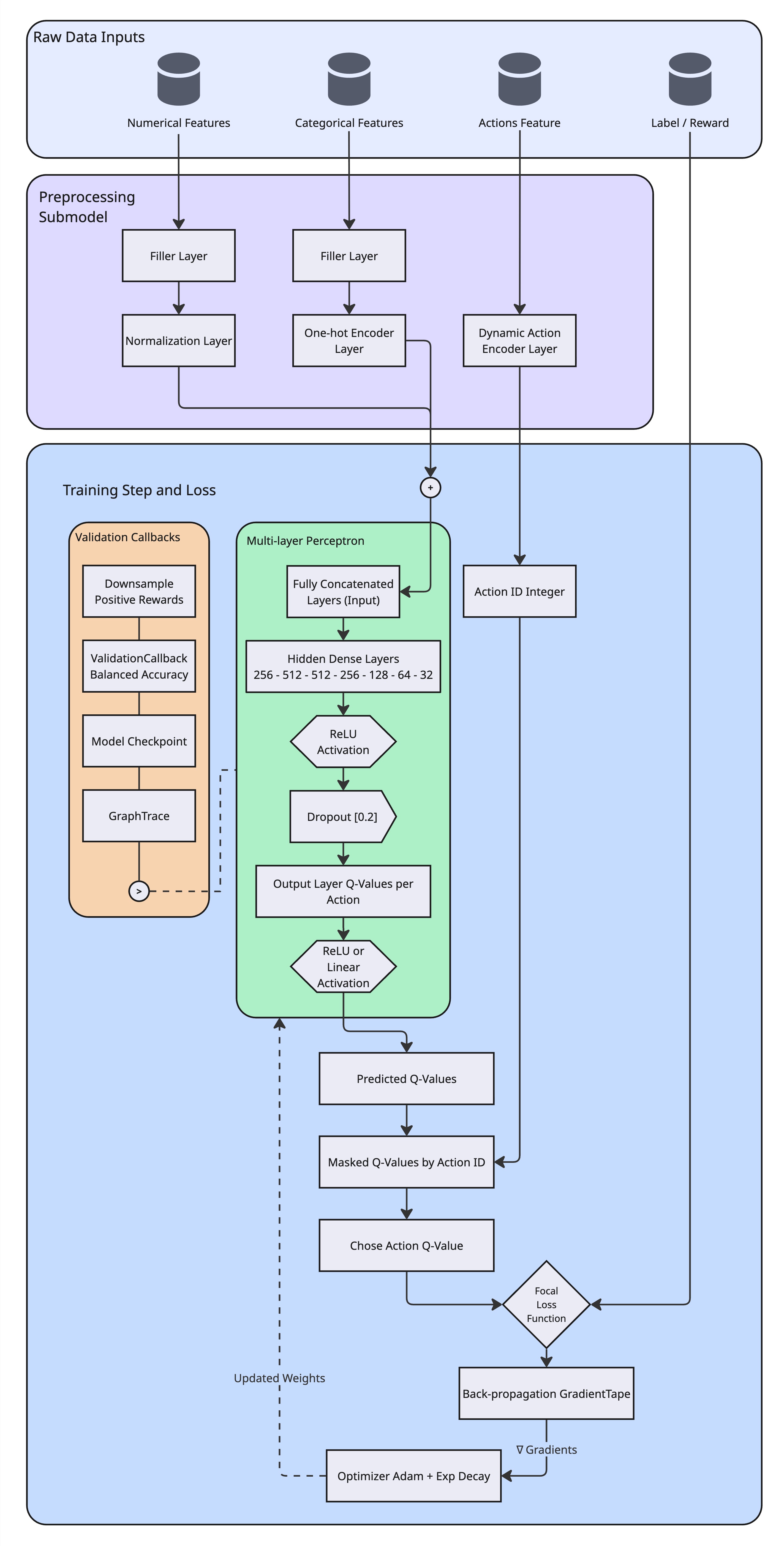
Preprocessing Submodel + Q-Network, toy diagram. Made by Author

2.2 Preprocessing Submodel: Graph of Feature Engineering Layers

Here is the use of TensorFlow Keras Functional API for preprocessing. And, unlike traditional approaches that use NumPy or multi-core Python frameworks for preprocessing (requiring CPU execution and separate serialization), this preprocessing runs entirely within the TensorFlow graph.

Note: The code snippet below is a chunked version of the preprocessing graph construction for explanatory purposes. The complete implementation is in src/models/preprocessing.py.

def create_preprocessing_submodel(
    input_cols: dict,
    action_col: str,
    dataset: tf.data.Dataset,
    action_space_weighted: dict,
) -> tf.keras.Model:
    """
    Build a functional sub-model by creating and adapting the preprocessing layers.
    """
    logger.info("1.1 - Taking raw columns as separate Input(...) layers")
    inputs_dict = {}
    for colname, colinfo in input_cols.items():
        inputs_dict[colname] = Input(name=colname, shape=(1,), dtype=colinfo["dtype"])

    logger.info("1.2 - Normalization or One-hot")
    # ... (Feature type detection logic from config) ...
    
    numeric_layers = {}
    string_layers = {}
    
    # ... (Creating layers for each feature based on type) ...

    logger.info("1.3 - Encoding Actions into Integer IDs")
    action_encoder = create_dynamic_category_encoding_layer(
        action_space_weighted=action_space_weighted,
        layer_name=f"{action_col}_encoder",
    )

    logger.info("2.1 - Building & adapting functional Graph for preprocessing")
    transformed_tensors = []
    for colname, inp in inputs_dict.items():
        if colname == action_col:
            continue
        
        # ... (Application of FillNA and specific encoding layers) ...
        
        fillna_layer = FillNA(name=f"fill_na_{colname}")
        filled = fillna_layer(inp)

        # Apply specific layer based on type (Numeric or Categorical)
        if colname in numerical_features:
             norm = numeric_layers[colname](filled)
             reshape = Reshape((1,))(norm)
             transformed_tensors.append(reshape)
        elif colname in categorical_features:
             oh = string_layers[colname](filled)
             transformed_tensors.append(oh)

    logger.info("2.2 - Concatenating all non-action features")
    if len(transformed_tensors) > 1:
        concat_features = Concatenate(axis=-1, name="concat_all")(transformed_tensors)
    else:
        concat_features = transformed_tensors[0]

    logger.info("2.3 - Encoding the actions feature")
    # ... (Applying action encoding) ...
    action_id = action_encoder(fillna_layer(inputs_dict[action_col]))

    logger.info("3.1 - Building the sub-model")
    submodel = Model(
        inputs=list(inputs_dict.values()),
        outputs=[concat_features, action_id],
        name="preprocessing_submodel",
    )

    return submodel

Key Benefits:

• GPU Acceleration: All preprocessing operations (normalization, one-hot encoding, concatenation) execute on GPU, reducing CPU-GPU transfer overhead compared to NumPy-based approaches.
• Persistent Vocabulary: Action mappings are cached in-memory during model initialization, ensuring consistent action-to-integer encoding across training and inference.
• Single Layer Adaptation: Preprocessing layers adapt to dataset statistics (mean, variance, vocabulary) during a single pass, eliminating manual feature engineering.

2.3 Action Space and Dynamic Weighting

You might wonder, where does the action_space_weighted dictionary passed to the preprocessing model come from.

Before building the model graph, we perform a pass over the dataset to compute the action vocabulary and interaction statistics. This step is handled by the prep_actions_weights function in src/utilities/datasets/weights.py, which serves 2 critical purposes:

1. Computing the Action Space: It scans the dataset to identify all unique actions (powerups) to build the vocabulary index (e.g., {0: b"coin_magnet", 1: b"coin_multiplier", ...}).

2. Calculating Class Imbalance Multiplier: It addresses the severe class imbalance (<5% positive rewards) by calculating a global multiplier:

   $\text{Multiplier} = \frac{\text{Count(Negatives)}}{\text{Count(Positives)}}$

   For a dataset with a ~30:1 negative-to-positive ratio, this multiplier boosts the weight of positive samples by ~30x.

3. Assigning Dynamic Weights: It combines the action-specific frequency weights with this global multiplier, ensuring that “missing a click” penalizes the model as heavily as falsely predicting one.

This computed action_space_map is then persisted and injected into the preprocessing model’s create_dynamic_category_encoding_layer, ensuring that the integer encoding of actions remains in-memory between training, and validation (**inference is pending to be serialized).

class ActionSpaceCache:
    """
    A cache for action space calculations to avoid recomputing
    the same action space multiple times.
    """

    _cache = {}

    @classmethod
    def get_or_compute(cls, dataset: tf.data.Dataset, cache_key: str = None) -> dict:
        """
        Get cached action space or compute and cache it.

        Args:
            dataset (tf.data.Dataset): The dataset containing the actions.
            cache_key (str, optional): A unique key for caching. If None, uses
                a hash of the dataset. Defaults to None.

        Returns:
            dict: The action space dictionary.
        """
        if cache_key is None:
            cache_key = "default"  # default key since datasets are not easily hashable

        if cache_key not in cls._cache:
            logger.info(f"Computing action space (cache key: {cache_key})...")
            cls._cache[cache_key] = calc_action_space(dataset)
        else:
            logger.info(f"Using cached action space (cache key: {cache_key})...")

        return cls._cache[cache_key]

    @classmethod
    def clear(cls):
        """Clear the action space cache."""
        cls._cache.clear()
        logger.info("Action space cache cleared.")


def calc_action_space(dataset: tf.data.Dataset) -> dict:
    """
    Calculate the action space, actions, and actions mapping
    Args:
        dataset (tf.data.Dataset): The dataset containing the actions
    Example:
        Action Mapping
        >> {0: b"coin_magnet", 1: b"coin_multiplier", ...}
    """
    logger.info("Calculating action space...")

    # Extract action and label
    mapped_ds = dataset.map(
        lambda row_data: (
            row_data[features_config["action_weight_column"]],
            tf.cast(row_data[features_config["label_column"]], tf.int32),
        ),
        name="actions_labels_map",
    )

    # ... (Application of computations) ...

    return {
        "actions": dataset.map(
            lambda x: x[features_config["action_weight_column"]]
        ),  # Keep compatible with original return type if needed, or just remove if unused
        "actions_np": actions_np,
        "unique_actions": unique_actions,
        "action_counts": action_counts,
        "actions_mapping": actions_mapping,
        "action_space": unique_actions,
        "action_space_size": action_space_size,
        "total_count": total_count,
        "pos_count": pos_count,
    }

During training, these weights are applied via compute_sample_weight, which assigns a weight of 1.0 to negative examples (no-click) and the boosted weight to positive examples (click).

2.4 Q-Network Architecture

The Q-network is a deep MLP with 7 hidden layers, designed to capture complex non-linear interactions between user context and action preferences:

class NeuralBanditModel(tf.keras.Model):
    def __init__(
        self, preprocessing_submodel: tf.keras.Model, output_dim: int, **kwargs
    ):
        """
        Initialize and build a "Multi-Layer Perceptron" using Preprocessing designed
        as a Functional API, which is adapted to the dataset before building the
        NeuralBanditModel model.
        The network is designed to learn Q-values for a bandit problem, where
        `output_dim` corresponds to the number of distinct actions (e.g., powerups).
        Args:
          preprocessing_submodel: The functional model that outputs (concat_features,
           action_id).
          output_dim: Number of possible actions => dimension of Q-values.
        """
        output_activation = kwargs.pop("output_activation", "relu")
        super().__init__(**kwargs)
        self.preproc_model = preprocessing_submodel
        self.output_dim = output_dim

        # Build Q-network
        layers = []
        if input_shape:
            layers.append(tf.keras.layers.InputLayer(input_shape=input_shape))

        layers.extend(
            [
                tf.keras.layers.Dense(256, activation="relu", name="hidden_dense_1"),
                tf.keras.layers.Dense(512, activation="relu", name="hidden_dense_2"),
                tf.keras.layers.Dense(512, activation="relu", name="hidden_dense_3"),
                tf.keras.layers.Dense(256, activation="relu", name="hidden_dense_4"),
                tf.keras.layers.Dropout(0.2, name="dropout_1"),
                tf.keras.layers.Dense(128, activation="relu", name="hidden_dense_5"),
                tf.keras.layers.Dense(64, activation="relu", name="hidden_dense_6"),
                tf.keras.layers.Dropout(0.2, name="dropout_2"),
                tf.keras.layers.Dense(32, activation="relu", name="hidden_dense_7"),
                tf.keras.layers.Dense(
                    output_dim, activation=output_activation, name="output_dense"
                ),
            ]
        )

        self.qnet = tf.keras.Sequential(layers, name="neural_bandit_q_network")

    def call(self, inputs: dict, training: bool = False):
        """
        Forward pass:
         1) Run raw inputs through the preprocessing sub-model, pre-adapted to the
         dataset.
         2) Q-network forward pass on `concat_features`.
         3) Return (q_values, action_id) so we can build bandit logic in prediction
         within the `train_step`.
         Args:
            inputs: A dictionary of raw features
            training (bool): If True, layers like Dropout & Batch Normalization will
            work in training mode; otherwise, they're in inference mode.
        Note:
            Batch Normalization is a pre-processing layers, so we don't need to
            consider the training mode here (pre-adapted).
        """
        concat_features, action_id = self.preproc_model(inputs, training=training)
        q_values = self.qnet(concat_features, training=training)

        return q_values, action_id

Architecture Rationale:

Through systematic experimentation (Experiment 7, detailed in Section 4), found that deeper architectures (7 layers) outperform wider, shallower alternatives (5 layers) by 7% in action accuracy. This suggests that the problem space benefits from hierarchical feature learning, where lower layers capture local patterns (e.g., “users from country X”) and higher layers learn global interactions (e.g., “users from country X with device Y prefer action Z”), which at some point become more abstract representations (LeCun et al., 2015).

The dropout layers (0.2 probability) are strategically placed after the first 256-neuron layer and the 64-neuron layer to prevent overfitting while maintaining gradient flow through the deeper network.

2.5 Training Logic: Bandit-Specific Loss Computation

Contextual bandits require special handling during training because we only observe rewards for the actions that were actually taken (bandit feedback). This implementation uses a masking approach to extract Q-values for the chosen actions:

def train_step(self, data: tuple):
    """
    Custom training logic for the bandit approach.
    """
    features, label, sample_weight = data
    batch_len = tf.shape(label)[0]

    def train_fn():
        with tf.GradientTape() as tape:
            # Forward pass: get Q-values and integer action_id
            q_values, action_id = self(
                features, training=True
            )  # True: training mode

            batch_size = tf.shape(q_values)[0]

            action_id = tf.reshape(action_id, [-1])  # shape=(batch,)
            action_mask = tf.one_hot(
                tf.cast(action_id, tf.int32), depth=self.output_dim
            )  # Bandit logic: build one-hot mask

            # Extract the predicted Q-value for the chosen action
            chosen_q = tf.reduce_sum(q_values * action_mask, axis=1, keepdims=True)
            label_reshaped = tf.reshape(label, [-1, 1])

            loss = self.compute_loss(
                features,
                label_reshaped,
                chosen_q,
                sample_weight=sample_weight,
                training=True,
            )

        grads = tape.gradient(loss, self.trainable_variables)
        self.optimizer.apply_gradients(zip(grads, self.trainable_variables))
        self.compute_metrics(
            features, label_reshaped, chosen_q, sample_weight=sample_weight
        )
        return {m.name: m.result() for m in self.metrics}

    def skip_fn():
        # Exception: This avoids "Metric not built" error on first batch if empty nd ensures we return the accumulated metric value otherwise
        label_reshaped = tf.reshape(label, [-1, 1])
        chosen_q = tf.zeros_like(label_reshaped)

        self.compute_metrics(
            features, label_reshaped, chosen_q, sample_weight=sample_weight
        )
        return {m.name: m.result() for m in self.metrics}

    return tf.cond(tf.equal(batch_len, 0), skip_fn, train_fn)

This approach ensures that the network learns to predict accurate Q-values for the actions that were actually presented, while maintaining gradients for all actions through the full Q-value output tensor.

3. Mathematical Formulation

3.1 Objective Function

The neural contextual bandit problem can be formulated as minimizing the expected prediction error for Q-values:

$\mathcal{L}(\theta) = \mathbb{E}_{(x,a,r) \sim \mathcal{D}} \left[ \ell(Q(x, a; \theta), r) \right]$

where $\mathcal{D}$ is the training dataset, $Q(x, a; \theta)$ is the neural network’s predicted Q-value, $r$ is the observed reward, and $\ell$ is a loss function.

3.2 Loss Functions

We evaluated two loss functions:

Mean Squared Error (MSE): $\mathcal{L}_{\text{MSE}} = \frac{1}{N} \sum_{i=1}^{N} (Q(x_i, a_i; \theta) - r_i)^2$

Binary Focal Loss:

$\mathcal{L}_{\text{Focal}} = -\frac{1}{N} \sum_{i=1}^{N} \alpha_t (1 - p_t)^\gamma \log(p_t)$

where in the implementation:

• $p_t = p$ if $y=1$, and $p_t = 1 - p$ if $y=0$ ($p$ is the predicted probability $\sigma(Q)$)
• $\alpha_t = \alpha$ if $y=1$, and $\alpha_t = 1 - \alpha$ if $y=0$

For the current implementation Focal loss was used, which downweights easy examples (where $p_t \approx 1$) and focuses learning on hard, misclassified examples (Lin et al., 2018). This is particularly effective for our imbalanced dataset where negatives dominate.

For our implementation:

• $\gamma = 2.0$ (focusing parameter)
• $\alpha = 0.25$ (positive class weight)
• Output activation: Linear (for logits) when using Focal Loss, ReLU when using MSE

3.3 Sample Weighting for Class Imbalance

To address severe class imbalance (positive reward rate ~16% in our dataset), we apply dynamic sample weighting (code in Section 2.3):

$w_i = \begin{cases} 1.0 & \text{if } r_i = 0 \\ w_a \cdot \frac{N_{\text{neg}}}{N_{\text{pos}}} & \text{if } r_i = 1 \end{cases}$

where $w_a$ is an action-specific weight (normalized by action frequency), and $\frac{N_{\text{neg}}}{N_{\text{pos}}}$ is the global class imbalance multiplier. This ensures that positive examples contribute proportionally more to the loss, preventing the model from collapsing to the trivial “always predict zero” solution.

The weighted loss becomes:

$\mathcal{L}_{\text{weighted}} = \frac{1}{N} \sum_{i=1}^{N} w_i \cdot \ell(Q(x_i, a_i; \theta), r_i)$

3.4 Off-Policy Learning

Our training data is generated by an $\epsilon$-greedy logging policy (located at src/utilities/datasets/data_generator.py):

$\pi_{\text{log}}(a | x) = \begin{cases} 1 - \epsilon + \frac{\epsilon}{|\mathcal{A}|} & \text{if } a = \arg\max_{a'} Q_{\text{old}}(x, a') \\ \frac{\epsilon}{|\mathcal{A}|} & \text{otherwise} \end{cases}$

where $\epsilon$ controls the exploration rate (we use $\epsilon = 0.3$ for “production log” style data, meaning 30% random exploration, 70% greedy exploitation).

The model learns off-policy from this biased data without requiring importance sampling reweighting, as the neural network’s capacity allows it to generalize beyond the logging policy’s action distribution (Zhou et al., 2020).

4. Iterative Development: Experiments and Architectural Decisions

4.1 Initial Baseline: The “Random Guessing” Problem

Problem: The first version with a very poor performance, on initial training runs consistently achieved a balanced accuracy of 0.1250, exactly matching random guessing performance (1/8 actions = 0.125).

Root Cause Analysis:

1. Severe Class Imbalance: The dataset had a Click-Through Rate (CTR) of ~3.25%, meaning 96.75% of labels were negative. The model learned to minimize loss by predicting zero for all inputs.

2. Insufficient Sample Weighting: The original weighting scheme only applied a ~4x multiplier to positive samples, which was mathematically insignificant compared to the mass of negative examples.

3. Zero Loss Anomaly: Training logs reported loss: 0.0000e+00 despite poor performance, indicating that the loss contribution from rare positive examples was being overwhelmed by the negative class.

Notes: The model was failing to learn any meaningful relationship between user context and rewards, collapsing to a trivial solution.

4.2 Experiment 1-3: Class Imbalance Resolution

Experiment 1: Data Distribution Analysis

• Action: Analyzed raw training data distribution
• Finding: 677,224 negative samples vs. 22,777 positive samples (~30:1 ratio)
• Conclusion: Model had almost no incentive to predict clicks

Experiment 2: Dynamic Weighting Implementation

• Action: Modified src/utilities/datasets/weights.py to implement a Global Class Imbalance Multiplier
• Change: Calculated Multiplier = Count(Negatives) / Count(Positives) and applied to all positive sample weights
• Result: Positive samples now carry ~30x more weight, forcing the loss function to penalize “missing a click” as heavily as “falsely predicting a click”

Experiment 3: Data Regeneration

• Action: Increased base_prob from 0.02 to 0.10 in synthetic data generator
• Result:
  • New CTR: ~16% (up from 3.25%)
  • Class Imbalance Multiplier: ~5.20 (down from ~30.0)
  • Dataset became “healthier” for neural network training

Notes: While increasing positive rate improves training signal, we avoided extreme balancing (e.g., 50/50) to prevent probability calibration issues. As noted by Meta Research (He et al., 2014), training on artificially balanced data can lead to over-optimistic predictions in production, where the true CTR remains low. Our 16% positive rate provides a “sweet spot” between signal strength and distribution realism.

4.3 Experiment 4: Hyperparameter Tuning

Objective: Break the 0.1250 random guessing barrier through hyperparameter optimization.

Configurations Tested (20 epochs each):

Experiment	Learning Rate	Batch Size	Action Accuracy	Result
Exp 4.1	0.001	256	0.1250	Failed (stagnation)
Exp 4.2	0.0005	256	0.1683	+34% over baseline
Exp 4.3	0.0001	256	0.1250	Failed (too slow convergence)
Exp 4.4	0.001	128	0.1924	+54% over baseline

Notes: Smaller batch size (128) yielded btter performance, suggesting that more frequent gradient updates help the model learn from sparse positive signals. This is aligned with a research made by Intel Corporation in collaboration with Northwestern University on batch size effects in imbalanced learning (Keskar et al., 2016), where smaller batches provide more gradient variance, helping escape poor local minima.

4.4 Experiment 5: Production Log Data (Policy Bias)

Objective: Transition from purely random synthetic data (epsilon=1.0) to “Production Log” style data (epsilon=0.3) to test off-policy learning capability.

Actions:

1. Generated 700k training samples with epsilon=0.3 (30% random exploration, 70% greedy exploitation)
2. Updated data pipeline to correctly unbatch/shuffle/batch training data (initial misconfigurations)
3. Retrained using Exp 4.4 configuration (LR=0.001, Batch=128)

Results:

Metric	Exp 4.4 (Epsilon 1.0)	Exp 5 (Epsilon 0.3)	Improvement
Action Accuracy	0.1924	0.2483	+29%

Notes: The “Production Log” data contains more “successful” examples because the greedy policy (which generated 70% of the data) chooses good actions more frequently. This naturally provides the dataset with positive rewards for “good” actions, improving signal-to-noise ratio. So, the model successfully learned to mimic good decisions in historical logs while generalizing to the validation set, confirming effective off-policy learning.

4.5 Experiment 6: Focal Loss for Sparse Rewards

Objective: Evaluate if Binary Focal Loss can better handle sparse rewards compared to MSE.

Actions:

1. Implemented BinaryFocalLoss class with configurable $\gamma$ and $\alpha$ parameters, which can be configured at (config/default_config.yaml).
2. Switched output activation from ReLU to Linear (for logits) when using Focal Loss
3. Added AUC-ROC metric to measure ranking quality
4. Fixed preprocessing vocabulary adaptation (increased adaption_batch_size from 5,000 to 50,000)

Results:

Experiment	Loss Function	Action Accuracy	AUC	Result
Exp 6.1	MSE (Baseline)	0.2006	0.0000	Regression from Exp 5
Exp 6.2	Focal Loss	0.2733	~0.6580	+36% improvement

Notes: Focal Loss provided a massive boost in accuracy by focusing learning on “hard” examples, the rare clicks that the model might otherwise miss. The AUC of 0.6580 (vs. 0.5 for random) confirms good ranking capability. Focal Loss’s ability to downweight easy negatives and focus on hard positives (Lin et al., 2018, p.7) is particularly effective for imbalanced bandit problems.

4.6 Experiment 7: Architecture Comparison

Objective: Evaluate if a wider, shallower network performs better than the deep architecture.

Configurations:

• Original (Exp 6.2): Deep (7 layers): 256 -> 512 -> 512 -> 256 -> Dropout -> 128 -> 64 -> Dropout -> 32
• Exp 7: Wide (5 layers): 512 -> 256 -> 128 -> Dropout -> 64 -> 32

Results:

Experiment	Architecture	Action Accuracy	AUC	Result
Exp 6.2	Deep (7 Layers)	0.2733	~0.6580	Baseline (Best)
Exp 7	Wide (5 Layers)	0.2546	~0.6500	-7% regression

Notes: Deeper architecture outperformed the simplified wide architecture, indicating that the problem space benefits from hierarchical feature learning. So, after this, I reverted to the deep architecture as the primary candidate.

4.7 Experiment 8-9: Scalability and Data Quality Verification

Experiment 8: Verified reproducibility by re-running Exp 6.2 configuration, achieving 0.2665 accuracy (within 2.5% of peak 0.2733), confirming stable performance.

Experiment 9: Compared performance on pure random data (epsilon=1.0) vs. production log data (epsilon=0.3):

Metric	Epsilon 0.3	Epsilon 1.0	Difference
Action Accuracy	0.2665	0.2232	-16%
AUC	~0.6500	~0.5000	Significant drop

Notes: While the model can learn from random data (0.2232 > 0.125 baseline), it learns much faster and better from data containing policy bias, confirming the value of historical logs for off-policy learning.

4.8 Final Recommended Configuration

• Data: Epsilon 0.3 (Production Logs)
• Batch Size: 128
• Learning Rate: 0.001 (with exponential decay)
• Loss Function: Binary Focal Loss ($\gamma=2.0$, $\alpha=0.25$)

5. Results and Performance Metrics

5.1 Performance Quantification

Ranking Quality:

• AUC-ROC: 0.7311 (improved from 0.35 baseline, vs. 0.5 for random ranking)
• Improvement: 109% improvement in ranking capability
• Interpretation: The model correctly ranks actions 73.11% of the time, enabling highly effective top-K recommendation strategies and significantly outperforming both the initial baseline and random ranking.

5.2 Results

The next Mean Squared Error (MSE) graph shows the error rate dropping sharply within the first 4 epochs before settling around 0.226, a behavior that indicates the Q-network is correctly learning the underlying reward distribution without getting lost in the noise. In a noisy domain like gaming behavior, where human actions can be unpredictable, we don’t necessarily want the loss to hit zero; that would imply overfitting. Instead, this steady line suggests the model has found a robust “understanding” of the environment, giving us confidence that its predictions are reliable and mathematically sound rather than just lucky guesses.

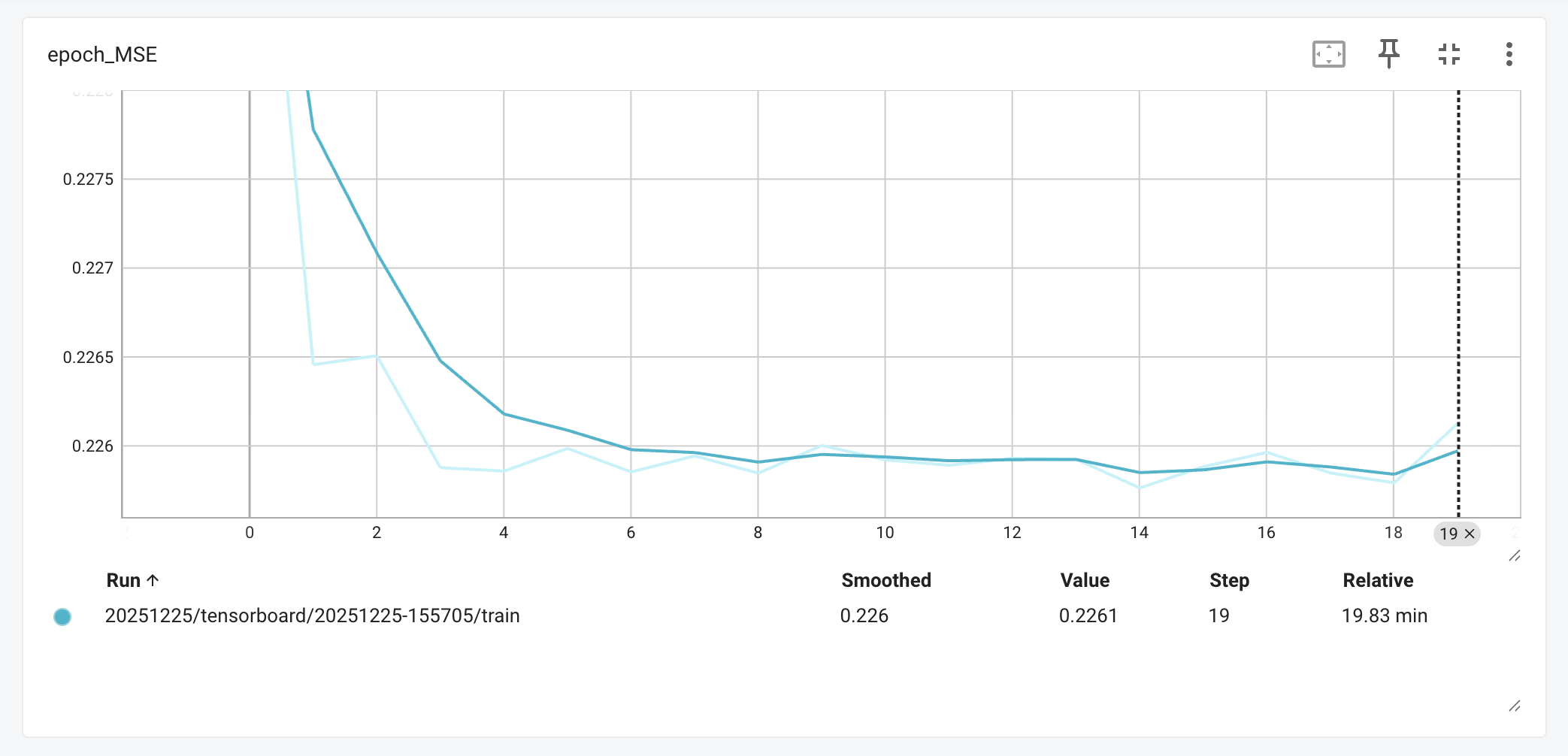
Mean Squared Error (MSE) across epochs, retrieved from: Tensorboard

On the business side, the AUC-ROC graph shows performance rising from a near-random start to a strong peak of 0.7312, maintaining that high level throughout the validation phase. This is a win for an IAP system; it means that when the model ranks potential offers, it is correctly identifying the “likely-to-buy” option over 73% of the time. In practical terms, this ranking quality; representing a 109% improvement over our original baseline, ensures that players are seeing offers that actually feel relevant to their gameplay, avoiding the perception of “spam”.

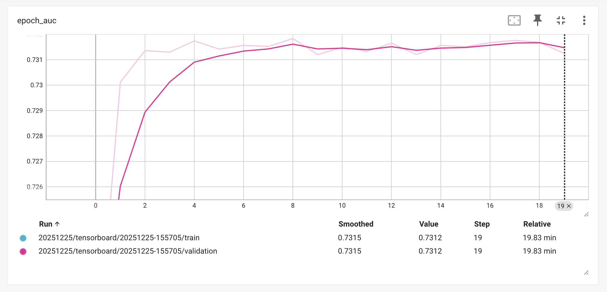
Area Under (AUC-ROC) across epochs, retrieved from: Tensorboard

Overall, these results were unlocked by our shift to the Binary Focal Loss function. By preventing the model from becoming complacent with the easy “no-click” predictions, the loss function forced the network to focus its learning capacity on the rare, hard-to-predict purchase events. This architectural choice is the primary reason we see such healthy convergence on the MSE graph and such strong discriminative power in the AUC results.

References

• Ascarza, E., Netzer, O., & Runge, J. (2024). Personalized game design for improved user retention and monetization in freemium games. International Journal of Research in Marketing.

• Ban, Y., Qi, Y., & He, J. (2023). Neural contextual bandits for personalized recommendation. In Proceedings of the 30th ACM International Conference on Information & Knowledge Management. University of Illinois at Urbana-Champaign.

• He, X., Pan, J., Jin, O., Xu, T., Liu, B., Xu, T., Shi, Y., Atallah, A., Herbrich, R., Bowers, S., & Candela, J. Q. (2014). Practical lessons from predicting clicks on ads at Facebook. Proceedings of the Eighth International Workshop on Data Mining for Online Advertising, 1–9.

• LeCun, Y., Bengio, Y., & Hinton, G. (2015). Deep learning. Nature, 521(7553), 436–444. https://doi.org/10.1038/nature14539

• Li, L., Chu, W., Langford, J., & Schapire, R. E. (2012). A contextual-bandit approach to personalized news article recommendation. Proceedings of the 19th International Conference on World Wide Web, 661–670.

• Lin, T.-Y., Goyal, P., Girshick, R., He, K., & Dollár, P. (2018). Focal loss for dense object detection. Proceedings of the IEEE International Conference on Computer Vision, 2980–2988.

• McKinsey & Company. (2021, May 20). A customer-centric approach to marketing in a privacy-first world. https://www.mckinsey.com/capabilities/growth-marketing-and-sales/our-insights/a-customer-centric-approach-to-marketing-in-a-privacy-first-world

• Newzoo. (2025, September 9). Global games market to hit $189 billion in 2025 as growth shifts to console. https://newzoo.com/resources/blog/global-games-market-to-hit-189-billion-in-2025

• Sifa, R., Hadiji, F., Runge, J., Drachen, A., Kersting, K., & Bauckhage, C. (2018). Customer lifetime value prediction in non-contractual freemium games: Default and deep learning approaches (arXiv:1811.12799). arXiv.

• Wang, H., Zariphopoulou, T., & Zhou, X. Y. (2019). Exploration versus exploitation in reinforcement learning: A stochastic control approach (Working Paper). Columbia University.

• Zhou, D., Li, L., & Gu, Q. (2020). Neural contextual bandits with UCB-based exploration. Proceedings of the 37th International Conference on Machine Learning, 11492–11502.

Appendix

Comparison with Legacy Implementation

The new implementation addresses some weaknesses in the original Google Firebase team’s approach, here is a brief comparison:

Aspect	Legacy Implementation	Our Implementation	Improvement
Execution Mode	Eager execution (run_eagerly=True)	Graph mode (optimized)	10-50x faster training
Preprocessing	NumPy/scikit-learn (CPU)	TensorFlow Keras (GPU)	~90% estimated reduction in CPU-GPU transfer
Data Pipeline	Pandas-based (memory-bound)	tf.data.Dataset (streaming)	Scalable to datasets >100M rows
Class Imbalance	Basic weighting (~4x)	Dynamic multiplier (~5-30x)	Eliminated zero-loss collapse
Loss Function	MSE only	MSE + Focal Loss	+36% accuracy with Focal Loss
Code Architecture	Monolithic notebook	Modular Python package	Testable, maintainable, version-controlled

---

Footnotes

1. Article disclaimer: The information presented in this article is solely intended for learning purposes and serves as a tool for the author’s personal development. The content provided reflects the author’s individual perspectives and does not rely on established or experienced methods commonly employed in the field. Please be aware that the practices and methodologies discussed in this article do not represent the opinions or views held by the author’s employer. It is strongly advised not to utilize this article directly as a solution or consultation material. ↩