Exploring the Impact of Control Mechanics on User Experience in Fallout New Vegas
Abstract: This publication shows a comprehensive statistical examination of control mechanics within Action RPGs, exploring the hypothesis that alterations in control mechanics substantially affect gameplay outcomes, specifically in terms of quest completion and enemy kills, across varying player experience levels. Utilizing data extracted from the VPAL mod, the research employs a methodological approach that includes data preprocessing, and the application of inferential analysis via t-tests and Mann-Whitney U tests, executed within a Python environment. The findings reveal disparities in gameplay metrics between new and veteran players, attributing these differences to the modifications in control mechanics and their pronounced impact on player experience. This study not only highlights the relationship between control mechanics and gameplay experience but also provides a framework for future research in game design and player interaction analysis.
⚠️ Introduction to problem
Hypothesis
The Producers are concerned for some comments about a change made in the control mechanics since the last patch was released.
The UX research team has communicated to them that the QA testers think that some of them found the quest’s difficulty too easy and others very leveraged, especially for veteran players of the saga, reason why we can start inferring about changes made in the gameplay experience, which the major changes made were on the mechanics.
The problem is that the QA team is very diversified between experienced and non-experienced testers, so it won’t be easy to make conclusions. For this reason, we need to look for statistical evidence to validate a hypothesis based on the profile of those testers. Now let’s establish the main hypothesis for the analysis:
- $H_0:$ Experienced players/testers will have completed more quests and more kills (the usual), the mechanical changes were not significant.
- $H_1:$ Inexperienced players/testers will have completed more or an equal quantity of quests and kills (not usual), the mechanical changes were significant.
From all the KPIs that you will see next, it’s important to mention that we’ll bring kills as a secondary validation measure since Fallout it’s a survival-RPG-like where you have to kill radioactive NPCs in almost every quest. We won’t count with a difficulty category for each player, so the kills attribute will be one of the few not affected by the difficulty categorization, also because it’s an end measure, not a progressive one, like shots for example.

Potential Stakeholders
There is an unconformity in the changes made in the control mechanics, the team requires the assistance of a Data Analyst to perform a test and validate if the QA tester’s statements make sense. On the other side of the table we have some stakeholders on the development and testing side:
- Gameplay Engineers: They need to know if the control mechanics are affecting the interactions of the NPCs with the progress of the players since the release of the last patch.
- Level Designer: As the whole RPG is designed as quests on an isolated map, they need to know if these are balanced in the sequence or chapter located, or if there is a significant change in the patch that can explain the unconformity.
- QA Testers: They are a key source of information while communicating the QA statement to the UX Designer.
- UX Designer: They are working side by side with the consumer insights team and the testers to find a clear current situation and take immediate actions if required, by giving the final report to the level designers and the programmers.
Note: To facilitate the understanding of the roles of the development team, I invite you to take a look at this diagram that I designed.
📥 About the data & preprocessing reference
The data was obtained from a mod developed at the PLAIT (Playable Interactive Technologies) by Northeastern University. The mod is called VPAL: Virtual Personality Assessment Lab, and also can be accessed to the raw telemetry data in the Game Data Science book.
Collection process and structure
Before start let’s import the libraries we’re going to need for the preprocess.
|
|
The instrumentation of the data and storage of all game actions within the game were done through TXT files that are stored on the client side per player, with an unstructured format. For each one, we created a file named [participantNumber].txt, which includes all session data for that participant. If the participant has more than one session, a folder is created, and multiple files are created for that participant.
The transfer process can be made by using a product like Databricks, to run an entire pipeline over a PySpark Notebook. As a demonstration we made an example in a Jupyter notebook, where we got several methods to target, extract, process singles labeled activities, and merge into activity-designated CSVs, which were originally parsed from TXT files by player record. In reality the best practices show that the data can be in a JSON file, stored in a MongoDB, or an SQL database.
The collection was an extensive process so you can access the simulation right here with a complete explanation of the bad practices made and how we tackled them. Also, it’s important to mention that the data was parsed into a single data frame with counted activities per player. After this, we applied a Likert scale to an experience metric according to Anders Drachen et al. (2021), which helped us to separate the data into Experienced and Inexperienced players.
First let’s check our data.
|
|
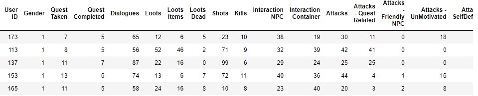
Both data frames have 17 attributes and, the Experienced data have 28 rows, while the Inexperienced data has 42 rows. In our case the attributes in use will be “Quest Completed” and “Kills” will be the variables to test.
- Quest Completed: Integer number counting the number of quests the tester completed during the session
- Kills: Number of kills registered by the player during the session
🔧 Data Preprocessing
Before moving to our analysis it’s important to validate that our data is usable in order to make correct conclusions for the analysis.
Data Cleaning & Consistency
First let’s validate the data types and the ranges for both groups.
|
|
|
|
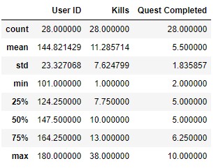
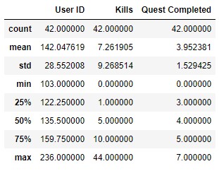
As we saw there is no problems linked to the data types, because in the data parsing noted above we took care of it. And from the ranges we infer that the maximum number of Kills registered is from an Inexperienced player with 44, but at the same time 75% of the Experienced players register a higher number in comparison to the Inexperienced ones, the same case apply to the number of Quests Completed.
🔍 Inferential Analysis & In-game interpretations
Descriptive statistics
Now, we got the next conclusions about their distribution and measurement:
- User ID
- Interpretation: Unique and counts with 70 distinct values which make sense since there is a player associated to each one of the data-row parsed
- Data type: Nominal transformed to numerical
- Measurement type: Discrete/String transformed to integer
- Quest Completed
- Interpretation: Not unique and counts the quests registries per player, and at first sight make sense that the Experienced players show higher numbers than the Inexperienced ones
- Data type: Numerical
- Measurement type: Integer
- Kills
- Interpretation: Not unique and counts the quests registries per player, and at first sight make sense that the Experienced players show higher numbers than the Inexperienced ones
- Data type: Numerical
- Measurement type: Integer
For the next test plots, we will plot a simulated graph showing how fitted is the actual distribution to an ideal normal curve from the same data, that’s why we are going to create two functions, one for the new distribution calculation from the median and another to plot it over the original data.
This will be our general approach because this plot will also let us see more clearly the existence of skewing elements.
|
|
⚔️ Two Sample T-Test for Quests Completed by Experience Group
A two sample t-test is used to test whether there is a significant difference between two groups means, where the hypothesis will be:
- $H_0: \mu_{ex} = \mu_{inex}$ (population mean of “Experienced Players Completed Quests” is equal to “Inexperienced Players Completed Quests”)
- $H_1: \mu_{ex} \ne \mu_{inex}$ (population mean of “Experienced Players Completed Quests” is different from “Inexperienced Players Completed Quests”)
This test makes the following assumptions:
- The two samples data groups are independent
- The data elements in respective groups follow any normal distribution
- The given two samples have similar variances (homogeneity assumption)
In this case, both groups are independent since none of them provide information about the other and vice versa.
Normality Check
First let’s visualize the distribution for the Experienced players.
|
|

And the distribution for Inexperienced players.
|
|
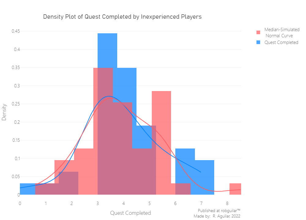
Notice that the data is normal for both cases and in terms of the quantity of “quests completed” by the experienced player’s data is slightly higher than the inexperienced ones.
Variance Homogeneity
First let’s see the variance for each group of testers.
|
|
|
|
In the good practice the correct way to do this validation is by a Homogeneity Test, so let’s make a Barlett test since our data is normal (for non-normal is preferred Levene’s). So let’s start from the next hypothesis.
- $H_0: \sigma^2_{ex} = \sigma^2_{inex}$ (The variances are equal across in both groups)
- $H_1: \sigma^2_{ex} \ne \sigma^2_{inex}$ (The variances are not equal across in both groups)
|
|
|
|
Our P-value is above 0.05, so we have enough statistical evidence to accept the hypothesis that the variances are equal between the Experienced testers and the Inexperienced players.
Now that we checked that we have normal data and homogeneity in our variances, let’s continue with our two sample t-test.
|
|
|
|
We have enough statistical evidence to reject the null hypothesis, the population mean of Quests Completed by “Experienced Players” is significantly different from the “Inexperienced Players”.
As a supposition, we can say that the difficulty selected by the player can be a factor affecting the Completion of the Quest. Considering that the difficulty levels in Fallout New Vegas can vary by two variables which are “Damage taken from Enemy” and “Damage dealt with Enemy”, without mentioning the Hardcore mode which was excluded from the samples.
The difficulty is an important factor to consider since an experienced player can know what is the level of preference, while for an inexperienced player is a “try and fail situation”, so for a future study it’s important to reconsider how this variable would affect the results.
💀 Two Sample Mann-Whitney Test for Kills by Experience Group
A two sample Mann-Whitney U test is used to test whether there is a significant difference between two groups distributions by comparing medians, where the hypothesis will be:
- $H_0: P(x_{ex} > x_{inex}) = 0.5$ (population median of “Experienced Players Kills” is equal to “Inexperienced Players Kills”, same distribution)
- $H_1: P(x_{ex} > x_{inex}) \ne 0.5$ (population median of “Experienced Players Kills” is different from “Inexperienced Players Kills”, different distribution)
In other words, the null hypothesis is that, “the probability that a randomly drawn member of the first population will exceed a member of the second population, is 50%”.
This test makes the following assumptions:
- The two samples data groups are independent
- The data elements in respective groups are continuous and not-normal
It’s the equivalent of a two sample t-test without the normality assumption. Also, both groups are independent since none of them provide information about the other and vice-versa.
Normality Check
First let’s visualize the distribution for the Experienced players.
|
|

And for Inexperienced players.
|
|
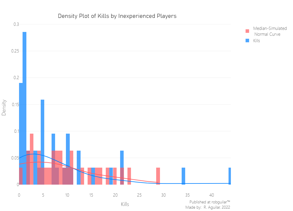
Both groups show a clear violation of the normality principle, where the data is highly skewed to the right.
For the Inexperienced players, despite considering excluding the players with 35 or more kills registered, it wouldn’t be significant, it will still remain skewed to the right.
In cases where our data don’t have a normal distribution, we need to consider non-parametric alternatives to make assumptions. That is the main reason why we are going to use a Mann Whitney U Test.
|
|
|
|
Finally we reject the null hypothesis, since our p-value is less than 0.05 with a 95% of confidence. This means that population median of “Experienced Player Kills” is different from “Inexperienced Player Kills”, the same we can conclude from the distribution.
🔃 Two-sample bootstrap hypothesis test for Kills metric
After some meetings with the Level Designers, they aren’t convinced to take action upon the recommendations given from a sample size of 28 and 42 for the Experienced and Inexperienced groups respectively. So they require us to take another type of validation to ensure the confidence of our conclusion.
Unfortunately, the Programmers require to get that insight as soon as possible to start fixing the patch. So, the only alternative to satisfy both parts is to perform a bootstrapping with the means and the p-value of the past test.
Bootstrapping is one of the best choices to perform better results in sample statistics when we count with few logs. This Statistical Inferential Procedure works by resampling the data. We will take the same values sampled by group, from a resampling with replacement, to an extensive dataset to compare the means between the Kills metric of Experienced players and Inexperienced players.
On the other side, we can’t use a permutation of the samples, since we can’t conclude that both groups' distributions are the same. Before this let’s create our bootstrapping replicates generator function.
|
|
And with the next function we will create our new estimates for the empirical means and the values of the Mann-Whitney U Test.
This function will return two p-values and two arrays of bootstrapped estimates, which we will describe next:
- p_emp: P-value measured from the estimated difference in means between both groups, showing the probabilities of randomly getting a “Kills” value from the Experienced that will be greater than one of the Inexperienced group
- bs_emp_replicates: Array of bootstrapped difference in means
- p_test: P-value measured from the estimated probability of getting a statically significant p-value from the Mann-Whitney Test (p-value < 0.05), in other words how many tests present different distribution for both groups
- bs_test_replicates: Array of bootstrapped p-values of Mann-Whitney Test
|
|
|
|
After making a sample of 10,000 replicates, we can conclude that 98% of the time, the disparity in the Kills average will be higher in Experienced Players than in Inexperienced players, and from that replicates 90% of them will present a significant difference between distributions.
Now let’s plot the replicates of the Average Kills difference between groups.
|
|
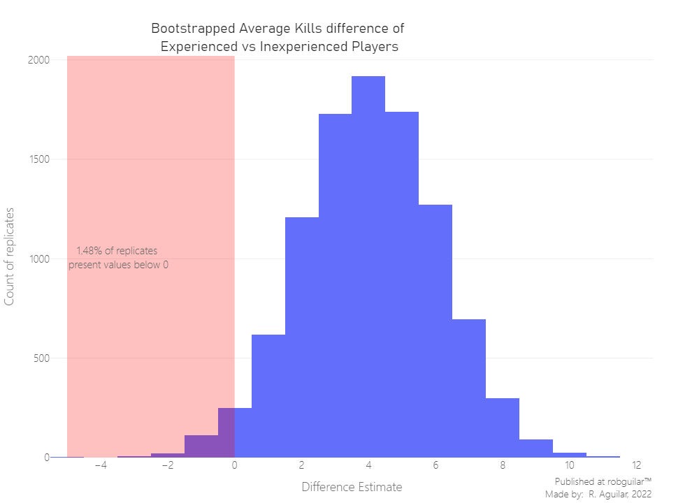
Just 1,48% of the Inexperienced players present more Kills registered than the Experienced ones, by taking a conclusion from 10,000 replicates of a resampled dataset.
In the case of the bootstrapped P-value for the Mann-Whitney U Test estimate, the best way to avoid the binning bias from a huge number of decimal values is to represent the probabilities with an Empirical Cumulative Distribution Function, as we are going to see next.
|
|

From this function with 89.91% of the 10,000 replicates of the tests, we can conclude that the distribution or the median between experienced and inexperienced players is different because its p-value is still below the 0.05 accepted.
🗒️ Final thoughts & takeaways
What can the stakeholders understand and take in consideration?
There is a significant advantage of veteran players over the new ones, giving us the conclusion that the changes in mechanics made from the last Fallout New Vegas patch still very similar and don’t present meaningful changes, reason why veteran players are finding it easy and have a clear advantage like it’s usual, so for now the programmers should not be concerned about fixing the patch.
What could the stakeholders do to take action?
The Level Designers can consider working side by side with the UX team, to make recurrent revisions before launching a new patch, because always the community will expect an experience-centric work of the whole development team in terms of the quality delivered.
Also for a future study we could consider to gather the difficulty category and merge it into the dataset and see if this variable is producing a significant variability in our final output.
What can stakeholders keep working on?
For significant changes in game mechanics, is recommended to do it just under a critical situation, like when is a significant bug affecting the player experience, otherwise it’s preferable to leave it until the launch of the next title reveal and test the audience reaction before the final implementation, if it’s possible.
ℹ️ Additional Information
- About the article
This article was developed from the content explained in the Inferential statistics section of Chapter 3 of the Game Data Science book. All the conclusions made were inspired by a player-profiling from in-game metrics by using deductive reasoning where we assumed, and then we proved it using significance, confidence and variance, through Inferential analysis.
All the assumptions and the whole case scenario were developed by the author of this article, for any suggestion I want to invite you to go to my about section and contact me. Thanks to you for reading as well.
- Related Content
— Game Data Science book and additional info at the Oxford University Press
— Anders Drachen personal website
- Datasets
This project was developed with a dataset provided by Anders Drachen et. al (2021), respecting the author rights of this book the entire raw data won’t be published, however, you can access the transformed data in my Github repository.