Abstract: This study explores the influence of adjusting the positioning of a “time gate” within the mobile game Cookie Cats, transitioning it from level 30 to level 40, on player retention rates. Predicated on the hypothesis that repositioning the gate would significantly impact user retention, the study gathered and analyzed data encompassing user IDs, game version details, rounds played, and retention metrics on the first and seventh days post-engagement. Employing exploratory data analysis alongside robust statistical methodologies, such as bootstrapping, to evaluate the collected data, the findings reveal a disparity in the retention rates on the first day, with a slight preference towards the control group, wherein the gate remained at level 30. This study contributes to the understanding of game design’s impact on player engagement and retention.

⚠️ Introduction to problem

Hypothesis

According to Rasmus Baath, Data Science Lead at castle.io, Tactile Entertainment is planning to move Cookie Cats' time gates from level 30 to 40, but they don’t know by how much the user retention can be impacted by this decision.

This sort of “time gate” is usually seen in free-to-play models, and normally contains ads that can be skipped using credits. In this case the player requires to submit a specific number of ‘Keys’, which also can be skipped in exchange of in-game purchases.

So seeing this viewpoint, a decision like this can impact not only user retention, the expected revenue as well that’s why we are going to set the initial hypothesis as:

• $H_0:$ Moving the Time Gate from Level 30 to Level 40 will decrease our user retention.
• $H_1:$ Moving the Time Gate from Level 30 to Level 40 will increase our user retention.

Potential Stakeholders

• Mobile Designer & User Retention Expert: They must be aligned with the final statement of the analyst, and make a final judgment to improve user retention.
• Level Designer: As the scene of levels is under study, the level designers need to take action on time to guarantee the storyline of the levels has a correct sequence, and to add it in a new patch.
• System Designer & System Engineer: If we extend the time gate, the credits should or should not remain at the same quantity required, which also needs to be implemented in the tracking system of the user progress.
• Executive Game Producer: As we mentioned before, a potential change requires a redesign of the earnings strategy and an alignment in the business expectation like funding, agreements, marketing, and patching deadlines.
• Players community: This stakeholder can be affected by the theory of hedonic adaptation, which is according to Rasmus Baath is “the tendency for people to get less and less enjoyment out of a fun activity over time if that activity is undertaken continuously”, meaning that if we prolong the time gate, this can affect the engagement in an unfavorable way, which in this case require an evaluation.

Note: To facilitate the understanding of the roles of the development team, I invite you to take a look at this diagram that I designed.

📥 About the data

Collection process and structure

Most of the time game developers work aside of telemetry systems, which according to Anders Drachen et al. (one of the pioneers in the Game Analytics field), from an interview made with Georg Zoeller of Ubisoft Singapore, the Game Industry manages two kinds of telemetry systems:

• Developer-facing: “The main goal of the system is to facilitate and improve the production process, gathering and presenting information about how developers and testers interact with the unfinished game”. Like the one mentioned in Chapter 7 of the “Game Analytics Maximizing the Value of Player Data” book, like the one implemented in Bioware’s production process of Dragon Age: Origins in 2009.
• User-facing: This one is “collected after a game is launched and mainly aimed at tracking, analyzing, and visualizing player behavior” mentioned in Chapters 4, 5, and 6 of the same book.

With the help of this kind of data-fetching system, we can create a responsive gate between the Data Analysts and the Designers. In most cases, these systems collect the data in form of logs (.txt) or dictionaries (.json), but fortunately in this case we will count with a structured CSV file.

1
2
3
4
5
6
7
8

# Importing pandas
import pandas as pd

# Reading in the data
df = pd.read_csv('datasets/cookie_cats.csv')

# Showing the first few rows
df.head()

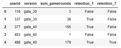
This dataset contains around 90,189 records of players that started the game while the telemetry system was running, according to Rasmus Baath. Among the variables collected are the next:

• userid : unique identification of the user.
• version : the group in which the players were measured, for a time gate at level 30 it contains a string called gate_30, or for a time gate at level 40 it contains a string called gate_40.
• sum_gamerounds : number of game rounds played within the first 14 days since the first session played.
• retention_1 : Boolean that defines if the player came back 1 day after the installation.
• retention_7 : Boolean that defines if the player came back 7 days after the installation.

Note: An important fact to keep in mind is that in the game industry one crucial metric is retention_1, since it defines if the game generate a first engagement with the first log-in of the player.

🔧 Data Preprocessing

Before starting the analysis we need to do some validations on the dataset.

1
2
3

# Count and display the number of unique players
print("Number of players: \n", df.userid.nunique(), '\n',
        "Number of records: \n", len(df.userid),'\n')

1
2
3
4

Number of players: 
 90188 
 Number of records: 
 90188

It’s not common to find this kind of data, cause as we saw the data is almost ideally sampled, where we count just with distinct records.

Data Cleaning

The data doesn’t require any kind of transformation and the data types are aligned with their purpose.

1

df.dtypes

1
2
3
4
5
6

userid             int64
version           object
sum_gamerounds     int64
retention_1         bool
retention_7         bool
dtype: object

Data Consistency

The usability of the data it’s rather good, since we don’t count with “NAN” (Not A Number), “NA” (Not Available), or “NULL” (an empty set) values.

 1
 2
 3
 4
 5
 6
 7
 8
 9
10
11
12
13
14
15

# Function the plot the percentage of missing values
def na_counter(df):
    print("NaN Values per column:")
    print("")
    for i in df.columns:
        percentage = 100 - ((len(df[i]) - df[i].isna().sum())/len(df[i]))*100

        # Only return columns with more than 5% of NA values
        if percentage > 5:
            print(i+" has "+ str(round(percentage)) +"% of Null Values")
        else:
            continue

# Execute function
na_counter(df)

1
2

NaN Values per column:
	None

By this way, we can conclude that there were not errors in our telemetry logs during the data collection.

Normalization

Noticing the distribution of the quartiles and comprehending the purpose of our analysis, where we only require sum_gamerounds as numeric, we can validate that the data is comparable and doesn’t need transformations.

1

df.describe()

🔍 Exploratory Analysis & In-game interpretations

Summary statistics

We got the next conclusions about their distribution and measurement:

• userid
  • Interpretation: Player identifier with distinct records in the whole dataset which can be transformed as a factor
  • Data type: Nominal
  • Measurement type: Discrete/String
• version
  • Interpretation: Just two possible values to evaluate, time gate at level 30 or level 40
  • Data type: Ordinal
  • Measurement type: Discrete/String
• sum_gamerounds
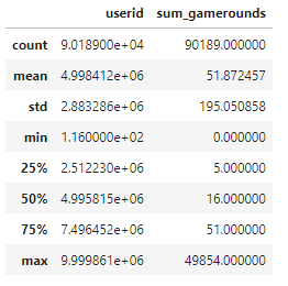
  • Interpretation: Number of game rounds played by the user, where 50% of the users played between 5 and 51 sessions
  • Data type: Numerical
  • Measurement type: Integer
• retention_1
  • Interpretation: Boolean measure to verify that the player retention was effective for 1 day at least
  • Data type: Nominal
  • Measurement type: Discrete/String
• retention_7
  • Interpretation: Boolean measure to verify that the player retention was effective for 7 days at least
  • Data type: Nominal
  • Measurement type: Discrete/String

Strategy of Analysis

The most accurate way to test changes is to perform A/B testing by targeting a specific variable, in the case retention (for 1 and 7 days after installation).

As we mentioned before, we have two groups in the version variable:

• Control group: The time gate is located at level 30. We are going to consider this one as a no-treatment group.
• Treatment group: The company plans to move the time gate to level 40. We are going to use this as a subject of study, due to the change involved.

In an advanced stage, we are going to perform a bootstrapping technique, to be confident about the result comparison for the retention probabilities between groups.

1
2
3
4
5
6

# Counting the number of players in each AB group.
players_g30 = df[df['version'] == 'gate_30']
players_g40 = df[df['version'] == 'gate_40']

print('Number of players tested at Gate 30:', str(players_g30.shape[0]), '\n',
     'Number of players tested at Gate 40:', str(players_g40.shape[0]))

1
2

Number of players tested at Gate 30: 44700 
 Number of players tested at Gate 40: 45489

Game rounds distribution

As we see the proportion of players sampled for each group is balanced, so for now, only exploring the Game Rounds data is in the queue.

Let’s see the distribution of Game Rounds (The plotly layout created is available in vizformatter library).

 1
 2
 3
 4
 5
 6
 7
 8
 9
10
11
12
13
14
15
16
17
18

import matplotlib.pyplot as plt
%matplotlib inline

import plotly.express as px

# Own layout design library
from vizformatter.standards import layout_plotly

# Load layout base objects
sign, layout = layout_plotly(height= 720, width= 1000, font_size= 15)

# Distribution Boxplot with outliers
box1 = px.box(df, x="sum_gamerounds",
            title = "Game Rounds Overall Distribution by player", labels = {"sum_gamerounds":"Game Rounds registered"})

box1.update_layout(layout)
box1.add_annotation(sign)
box1.show()

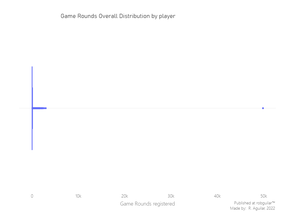
For now, we see that exist clear outliers in the dataset since one user has recorded 49,854 Game rounds played in less than 14 days, meanwhile, the max recorded, excluding the outlier, is around 2,900. The only response to this case situation is a “bot”, a “bug” or a “glitch”.

Nevertheless, it’s preferable to clean it, since only affected one record. Let’s prune it.

1

df = df[df['sum_gamerounds'] != 49854]

We can make an Empirical Cumulative Distribution Function, to see the real distribution of our data.

Note: In this case, we won’t use histograms to avoid a binning bias.

 1
 2
 3
 4
 5
 6
 7
 8
 9
10
11
12
13
14
15
16
17
18
19
20
21
22
23
24
25
26
27
28
29
30
31
32
33
34
35
36
37
38
39
40
41

import plotly.graph_objects as go

# Import numpy library
import numpy as np

# ECDF Generator function
def ecdf(data):
    # Generate ECDF (Empirical Cumulative Distribution Function)
    # for on dimension arrays
    n = len(data)

    # X axis data
    x = np.sort(data)

     # Y axis data
    y = np.arange(1, n+1) / n

    return x, y

# Generate ECDF data
x_rounds, y_rounds = ecdf(df['sum_gamerounds'])

# Generate percentile makers 
percentiles = np.array([5,25,50,75,95])
ptiles = np.percentile(df['sum_gamerounds'], percentiles)

# ECDF plot
ecdf = go.Figure()

# Add traces
ecdf.add_trace(go.Scatter(x=x_rounds, y=y_rounds,
                    mode='markers',
                    name='Game Rounds'))
ecdf.add_trace(go.Scatter(x=ptiles, y=percentiles/100,
                    mode='markers+text',
                    name='Percentiles', marker_line_width=2, marker_size=10,
                    text=percentiles, textposition="bottom right"))
ecdf.update_layout(layout)
ecdf.update_layout(title='Game Rounds Cumulative Distribution Plot', yaxis_title="Cumulative Probability")
ecdf.add_annotation(sign)
ecdf.show()

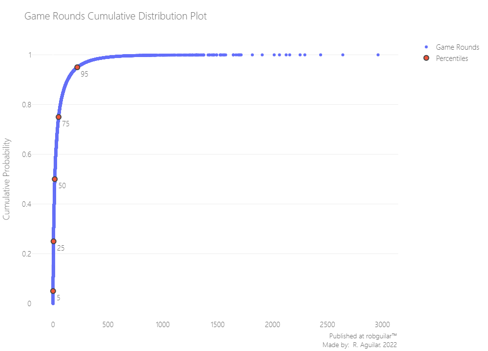
As we see 95% of our data is below 500 Game Rounds.

1
2

print("The 95 percentile of the data is at: ", ptiles[4], "Game Rounds","\n",
"This means ", df[df["sum_gamerounds"] <= ptiles[4]].shape[0], " players")

1
2

The 95 percentile of the data is at:  221.0 Game Rounds 
 This means  85706  players

For us, this can be considered a valuable sample.

In the plot above, we saw some players that installed the game but, then never return (0 game rounds).

1

print("Players inactive since installation: ", df[df["sum_gamerounds"] == 0].shape[0])

1

Players inactive since installation:  3994

And in most cases, players just play a couple of game rounds in their first two weeks. But, we are looking for players that like the game and to get hooked, that’s one of our interests.

A common metric in the video gaming industry for how fun and engaging a game is 1-day retention as we mentioned before.

📊 Player retention analysis

Retention is the percentage of players that come back and plays the game one day after they have installed it. The higher 1-day retention is, the easier it is to retain players and build a large player base.

According to Anders Drachen et al. (2013), these customer kind metrics “are notably interesting to professionals working with marketing and management of games and game development”, also this metric is described simply as “how sticky the game is”, in other words, it’s essential.

As a first step, let’s look at what 1-day retention is overall.

1
2
3
4

# The % of users that came back the day after they installed
prop = len(df[df['retention_1'] == True]) / len(df['retention_1']) * 100

print("The overall retention for 1 day is: ", str(round(prop,2)),"%")

1

The overall retention for 1 day is:  44.52 %

Less than half of the players come back one day after installing the game.

Now that we have a benchmark, let’s look at how 1-day retention differs between the two AB groups.

🔃 1-day retention by A/B Group

Computing the retention individually, we have the next results.

 1
 2
 3
 4
 5
 6
 7
 8
 9
10

# Calculating 1-day retention for each AB-group

# CONTROL GROUP
prop_gate30 = len(players_g30[players_g30['retention_1'] == True])/len(players_g30['retention_1']) * 100

# TREATMENT GROUP
prop_gate40 = len(players_g40[players_g40['retention_1'] == True])/len(players_g40['retention_1']) * 100

print('Group 30 at 1 day retention: ',str(round(prop_gate30,2)),"%","\n",
     'Group 40 at 1 day retention: ',str(round(prop_gate40,2)),"%")

1
2

Group 30 at 1 day retention:  44.82 % 
 Group 40 at 1 day retention:  44.23 %

It appears that there was a slight decrease in 1-day retention when the gate was moved to level 40 (44.23%) compared to the control when it was at level 30 (44.82%).

It’s a smallish change, but even small changes in retention can have a huge impact. While we are sure of the difference in the data, how confident should we be that a gate at level 40 will be more threatening in the future?

For this reason, it’s important to consider bootstrapping techniques, this means “a sampling with replacement from observed data to estimate the variability in a statistic of interest”. In this case, retention, and we are going to do a function for that.

 1
 2
 3
 4
 5
 6
 7
 8
 9
10

# Bootstrapping Function
def draw_bs_reps(data,func,iterations=1):
    boot_Xd = []
    for i in range(iterations):
        boot_Xd.append(func(data = np.random.choice(data, len(data))))
    return boot_Xd
# Retention Function
def retention(data):
    ret = len(data[data == True])/len(data)
    return ret

Control Group Bootstrapping

1
2

# Bootstrapping for gate 30
btg30_1d = draw_bs_reps(players_g30['retention_1'], retention, iterations = 1000)

Treatment Group Bootstrapping

1
2

# Bootstrapping for gate 40
btg40_1d = draw_bs_reps(players_g40['retention_1'], retention, iterations = 1000)

Now, let’s check the results

 1
 2
 3
 4
 5
 6
 7
 8
 9
10
11
12
13
14
15
16
17
18
19
20
21

import plotly.figure_factory as ff

mean_g40 = np.mean(btg40_1d)
mean_g30 = np.mean(btg30_1d)

# A Kernel Density Estimate plot of the bootstrap distributions
boot_1d = pd.DataFrame(data = {'gate_30':btg30_1d, 'gate_40':btg40_1d},
                       index = range(1000))

# Plotting histogram
hist_1d = [boot_1d.gate_30, boot_1d.gate_40]
dist_1d = ff.create_distplot(hist_1d, group_labels=["Gate 30 (Control)", "Gate 40 (Treatment)"], show_rug=False, colors = ['#3498DB','#28B463'])
dist_1d.add_vline(x=mean_g40, line_width=3, line_dash="dash", line_color="#28B463")
dist_1d.add_vline(x=mean_g30, line_width=3, line_dash="dash", line_color="#3498DB")
dist_1d.add_vrect(x0=mean_g30, x1=mean_g40, line_width=0, fillcolor="#F1C40F", opacity=0.2)

dist_1d.update_layout(layout)
dist_1d.update_layout(xaxis_range=[0.43,0.46])
dist_1d.update_layout(title='1-Day Retention Bootstrapping by A/B Group', xaxis_title="Retention")
dist_1d.add_annotation(sign)
dist_1d.show()

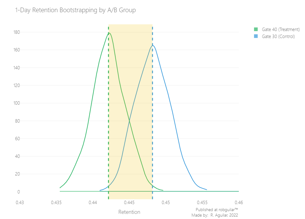
The difference still looking close, for this reason, is preferable to zoom it by plotting the difference as an individual measure.

 1
 2
 3
 4
 5
 6
 7
 8
 9
10
11
12
13
14
15

# Adding a column with the % difference between the two AB-groups
boot_1d['diff'] = (
                    ((boot_1d['gate_30'] - boot_1d['gate_40']) / boot_1d['gate_40']) * 100
                )

# Ploting the bootstrap % difference
hist_1d_diff = [boot_1d['diff']]
dist_1d_diff = ff.create_distplot(hist_1d_diff, show_rug=False, colors = ['#F1C40F'],
                                    group_labels = ["Gate 30 - Gate 40"], show_hist=False)
dist_1d_diff.add_vline(x= np.mean(boot_1d['diff']), line_width=3, line_dash="dash", line_color="black")
dist_1d_diff.update_layout(layout)
dist_1d_diff.update_layout(xaxis_range=[-3,6])
dist_1d_diff.update_layout(title='Percentage of "1 day retention" difference between A/B Groups', xaxis_title="% Difference")
dist_1d_diff.add_annotation(sign)
dist_1d_diff.show()

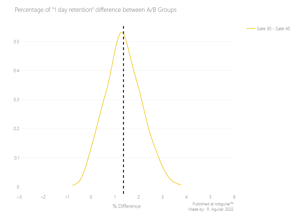
From this chart, we can see that the percentual difference is around 1% - 2%, and that most of the distribution is above 0%, in favor of a gate at level 30.

But, what is the probability that the difference is above 0%? Let’s calculate that as well.

1
2
3
4
5

# Calculating the probability that 1-day retention is greater when the gate is at level 30
prob = (boot_1d['diff'] > 0.0).sum() / len(boot_1d['diff'])

# Pretty printing the probability
print('The probabilty of Group 30 (Control) having a higher \n retention than Group 40 (Treatment) is: ', prob*100, '%')

1
2

The probabilty of Group 30 (Control) having a higher 
 retention than Group 40 (Treatment) is:  96.39999999999999 %

🔃 7-day retention by A/B Group

The bootstrap analysis tells us that there is a high probability that 1-day retention is better when the time gate is at level 30. However, since players have only been playing the game for one day, likely, most players haven’t reached level 30 yet. That is, many players won’t have been affected by the gate, even if it’s as early as level 30.

But after having played for a week, more players should have reached level 40, and therefore it makes sense to also look at 7-day retention. That is: What percentage of the people that installed the game also showed up a week later to play the game again?

Let’s start by calculating 7-day retention for the two AB groups.

1
2
3
4
5
6

# Calculating 7-day retention for both AB-groups
ret30_7d = len(players_g30[players_g30['retention_7'] == True])/len(players_g30['retention_7']) * 100
ret40_7d = len(players_g40[players_g40['retention_7'] == True])/len(players_g40['retention_7']) * 100

print('Group 30 at 7 day retention: ',str(round(ret30_7d,2)),"%","\n",
     'Group 40 at 7 day retention: ',str(round(ret40_7d,2)),"%")

1
2

Group 30 at 7 day retention:  19.02 % 
 Group 40 at 7 day retention:  18.2 %

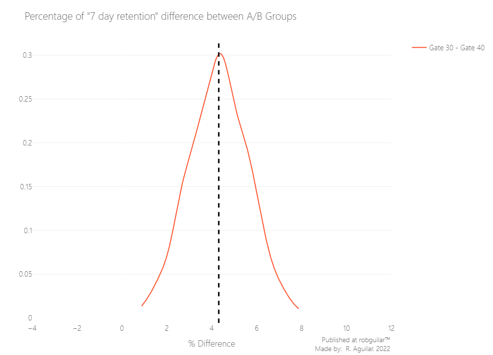
Like with 1-day retention, we see that 7-day retention is barely lower (18.20%) when the gate is at level 40 than when the time gate is at level 30 (19.02%). This difference is also larger than for 1-day retention.

We also see that the overall 7-day retention is lower than the overall 1-day retention; fewer people play a game a week than a day after installing.

But as before, let’s use bootstrap analysis to figure out how sure we can be of the difference between the AB-groups.

Control & Treatment Group Bootstrapping

 1
 2
 3
 4
 5
 6
 7
 8
 9
10
11
12
13
14
15
16
17
18
19
20
21
22
23
24
25
26
27
28
29
30

# Creating a list with bootstrapped means for each AB-group

# Bootstrapping for CONTROL group
btg30_7d = draw_bs_reps(players_g30['retention_7'], retention, iterations = 500)

# Bootstrapping for TREATMENT group
btg40_7d = draw_bs_reps(players_g40['retention_7'], retention, iterations = 500)

boot_7d = pd.DataFrame(data = {'gate_30':btg30_7d, 'gate_40':btg40_7d},
                       index = range(500))

# Adding a column with the % difference between the two AB-groups
boot_7d['diff'] = (boot_7d['gate_30'] - boot_7d['gate_40']) /  boot_7d['gate_30'] * 100

# Ploting the bootstrap % difference
hist_7d_diff = [boot_7d['diff']]
dist_7d_diff = ff.create_distplot(hist_7d_diff, show_rug=False, colors = ['#FF5733'],
                                    group_labels = ["Gate 30 - Gate 40"], show_hist=False)
dist_7d_diff.add_vline(x= np.mean(boot_7d['diff']), line_width=3, line_dash="dash", line_color="black")
dist_7d_diff.update_layout(layout)
dist_7d_diff.update_layout(xaxis_range=[-4,12])
dist_7d_diff.update_layout(title='Percentage of "7 day retention" difference between A/B Groups', xaxis_title="% Difference")
dist_7d_diff.add_annotation(sign)
dist_7d_diff.show()

# Calculating the probability that 7-day retention is greater when the gate is at level 30
prob = (boot_7d['diff'] > 0).sum() / len(boot_7d)

# Pretty printing the probability
print('The probabilty of Group 30 (Control) having a higher \n retention than Group 40 (Treatment) is: ~', prob*100, '%')

1
2

The probabilty of Group 30 (Control) having a higher 
 retention than Group 40 (Treatment) is: ~ 100.0 %

🗒️ Final thoughts & takeaways

What can the stakeholders understand and take in consideration?

As we underlined retention is crucial, because if we don’t retain our player base, it doesn’t matter how much money they spend in-game purchases.

So, why is retention higher when the gate is positioned earlier? Normally, we could expect the opposite: The later the obstacle, the longer people get engaged with the game. But this is not what the data tells us, we explained this with the theory of hedonic adaptation.

What could the stakeholders do to take action?

Now we have enough statistical evidence to say that 7-day retention is higher when the gate is at level 30 than when it is at level 40, the same as we concluded for 1-day retention. If we want to keep consumer retention high, we should not move the gate from level 30 to level 40, it means we keep our Control method in the current gate system.

What can stakeholders keep working on?

For coming strategies the Game Designers can consider that, by pushing players to take a break when they reach a gate, the fun of the game is postponed. But, when the gate is moved to level 40, they are more likely to quit the game because they simply got bored of it.

ℹ️ Additional Information

• About the article

With acknowledgment to Rasmus Baraath for guiding this project. Which was developed for sharing knowledge while using cited sources of the material used.

Thanks to you for reading as well.

• Related Content

For more content related to the authors mentioned, I invite you to visit the next sources:

– Anders Drachen personal website.

– Rasmus Baath personal blog.

– Georg Zoeller personal keybase.

Also in case you want to share some ideas, please visit the About section and contact me.

• Datasets

This project was developed with a dataset provided by Rasmus Baath, which also can be downloaded at my Github repository.